Render Modes

Each scenario can be rendered in up to three modes. The modes differ only in how investment returns are applied — everything else (income, spending, events, taxes) uses the same engine.

Deterministic Mode

The default. Start here.

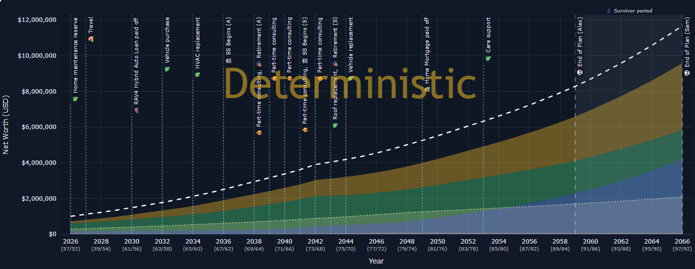
A single trajectory using fixed return assumptions from your scenario’s [assumptions] section:

• stock_return — expected annual stock return
• bond_return — expected annual bond return
• equity_allocation — percentage allocated to stocks (rest in bonds)
• inflation — annual inflation rate

The blended return is computed as: equity_allocation * stock_return + (1 - equity_allocation) * bond_return

Every year uses the same return. The result is a clean, single-line chart that’s easy to understand. Use this mode for most analysis and scenario comparison.

Best for: day-to-day planning, scenario comparison, what-if analysis.

Historical Mode

Runs the model against actual market return sequences from a bundled dataset (US balanced portfolio, 1926–present).

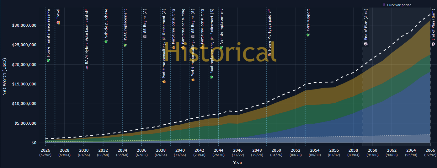
For each historical starting year in the dataset, the model runs a complete projection using that year’s actual stock and bond returns. The result shows what would have happened if your current situation had started in each of those historical periods.

The chart shows:

• The range of outcomes across all historical periods
• The median outcome
• Individual traces for specific historical periods

Best for: understanding how your plan would have fared in past market downturns (Great Depression, 2008, 2022).

Monte Carlo Mode

Runs thousands of simulations with randomized annual returns. Each simulation randomly samples returns from a normal distribution based on your stock_return, bond_return, and portfolio_return_volatility settings plus the equity_allocation.

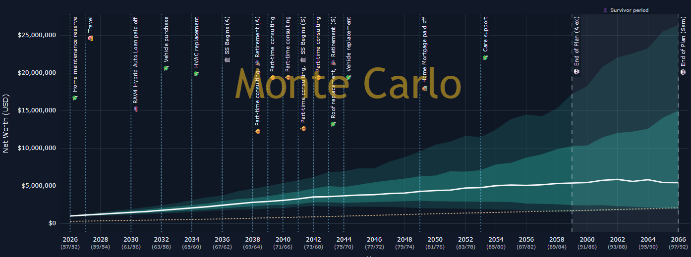
The chart shows:

• Shaded bands — the 10th–25th, 25th–50th, 50th–75th, and 75th–90th percentile ranges
• Median line — the 50th percentile outcome
• Transparency — darker areas show more likely outcomes

Success Metrics

The Simulation tab shows key metrics:

Metric	What It Tells You
Probability of Success	Percentage of simulations where the portfolio never drops below zero
Median Terminal NW	The middle-of-the-road ending net worth
Worst-Decile Terminal NW	The 10th percentile outcome — plan for this
First Failure Year	The earliest year where any simulation failed
Peak Pressure Rate	The highest percentage of simulations failing in a single year

Configuration

Monte Carlo behavior is configured in your scenario TOML under [monte_carlo.success]:

[monte_carlo.success]
failure_mode = "net_worth_below_zero"
minimum_spending_funded_ratio = 1.0
failure_grace_period_months = 6

Setting	What It Does
failure_mode	What counts as failure: net_worth_below_zero, liquid_depletion, spending_shortfall, or preserve_home_equity
minimum_spending_funded_ratio	For spending_shortfall mode — what fraction of spending must be covered
failure_grace_period_months	Short-term dips that resolve within this window don’t count as failure
num_runs	Number of Monte Carlo simulations (default: 1000)
seed	Random seed for reproducible results

Best for: stress-testing your plan against uncertainty, understanding probabilities, identifying risk years.

Choosing a Mode

If you want to…	Use
See a clean baseline	Deterministic
Understand how past crises would affect you	Historical
Quantify risk and uncertainty	Monte Carlo
Compare scenario A vs scenario B	Deterministic (cleanest comparison)
Present to a partner or advisor	Deterministic (clearest, least confusing)